Other Links:
|
- Algorithmic Information Theory
- Turing Machines and the Halting Problem
- Church-Turing Thesis
- Universal Turing Machines
- Kolmogorov Complexity
- Some Other Concepts
- Programs and Self-Delimiting Codes
- Selection of UTM
- Chaitin's Halting Probability: Omega
- References
- Links
Algorithmic Information Theory
Gregory Chaitin[1], Ray Solomonoff, and Andrei Kolmogorov developed a different view of information from that of Shannon. Rather than considering the statistical ensemble of messages from an information source, algorithmic information theory looks at individual sequences of symbols. Here, information H(X) is defined as the minimum size of a program necessary to generate the sequence X.
This article highlights some of the main concepts of Algorithmic Information Theory. Knowledge of this subject can be useful when arguing with Creationists whose use of concepts from both Classical and Algorithmic Information Theory might be sloppy. This article is only a survey of the major ideas. For the mathematical proofs and more detailed background, see the cited material and the links.
Turing Machines and the Halting Problem[Top]
Understanding Algebraic Information Theory requires knowledge of Turing Machines. Alan Turing[2] showed that it is possible to invent a single machine U capable of computing any computable sequence. Turing's notations are somewhat difficult, but the basic idea is as follows:
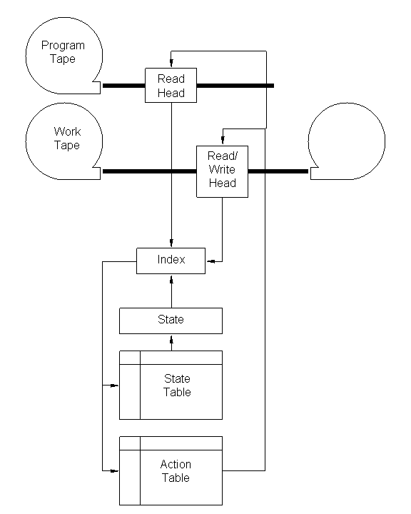
The elements of a Turing Machine are a program tape with a read head, a work tape with a read/write head, a state (represented by a number), a state table, and an action table. The program tape is of finite length and contains a sequence of symbols. The work tape is initially blank. For each machine cycle, the state is replaced by the look-up value in the state table. The look-up index is a combination of the current state, and the symbol read from the program tape, and the symbol read from the work tape.
The action table controls the tapes. The following actions are allowed:
- Halt
- Advance the program tape one symbol to the right
- Advance the work tape one symbol to the right
- Rewind the work tape one symbol to the left
- Erase the current symbol on the work tape
- Write any one of R symbols on the work tape (there are R of these actions).
We can think of the tapes on the Turing Machine as strings; that is, sequences of symbols. We will call the program string p, and the resulting output string on the work tape X. Program p produces string X on Turing Machine T. Given that we have Turing Machine T, string X can be represented by p. We can also think of p and X as numbers, since numbers are represented as symbol sequences.
Often, we are talking about binary Turing Machines, for which the symbol set on the two tapes is consists of 0 and 1. This need not be the case, however. We can have any number of symbols. Now obviously, we can't really have an infinitely long work tape, but the Turing Machine is used for theoretical problems so we can imagine that we do.
A diagram of a Turing Machine is shown below:
 |
For a good description of Turing Machines, see the Stanford Encyclopedia of Philosophy[3]. Note that theoretical Turing Machines have infinite work tapes, which of course cannot be constructed. Some problems are therefore not possible to run on actual, physical Turing Machines.
Turing invented his theoretical machine to address the Entscheidungsproblem or decision problem; that is, whether it is possible in symbolic logic to find a general algorithm which decides for given first-order statements whether they are universally valid or not.
The modern roots of the Entscheidungsproblem go back to a 1900 speech by David Hilbert. [4] Hilbert had hoped it would be possible to develop a general algorithm for deciding whether a set of axioms were self-contradictory. Kurt Gödel [5] showed that, in any axiomatic system for arithmetic on natural numbers, some propositions exist that cannot be proved or disproved within the axioms of the system. This is known as Gödel's Incompleteness Theorem, and it demonstrated that Hilbert's Second Problem could not be solved.
Turing, building on the work of Gödel, proved that the Entscheidungsproblemwas not solvable. Alonzo Church, independently of Turing, showed the same thing.
Turing used the halting problem for his proof. The halting problem is a decision problem. It poses the question: given a description of an algorithm and its initial conditions, can one show that the algorithm will halt? An algorithm producing the digits of πis an example of a non-halting algorithm π is an irrational and transcendental number; it cannot be expressed as a polynomial with rational coefficients and therefore has an infinite number of digits). Turing proved that no general algorithm exists that can solve the halting problem for all possible inputs, and hence that the Entscheidungsproblem is unsolvable.
Church-Turing Thesis [Top]
The Church-Turing Thesis is a synthesis of Church's Thesis and Turing's Thesis. It essentially states that, whenever, there is an effective method for obtaining the values of a mathematical function, the function can be computed by a Turing machine. The basic idea is that, if you have a calculation that can be computed by any (deterministic) machine that can be effectively implemented, a Turing machine can do the calculation.
Two competing views of the Church-Turing Thesis have been published by Copeland[6] and Hodges[7] (the argument is, at least in part, about how strongly stated a thesis Church and Turing would have agreed to, and whether they bought in to the concept described by Gandy as Thesis M).
Universal Turing Machine [Top]
It would not be practical to construct a new Turing Machine every time one wants to run a calculation, giving rise to the concept of Universal Turing Machine (UTM). A Universal Turing Machine (UTM) is defined as a Turing Machine that can simulate any other Turing Machine. If we have a UTM, we can program it to act like any Turing Machine we want.
Since a Turing Machine can be described by its state and action tables, it can be represented as a string. If p is a program on a Turing Machine T that produces string X on the work tape, then on a Universal Turing Machine we can load a string representation of T, run program p, and get X. We will use symbol u for the representation of T on U. Therefore, if <u><p> is input to U, it outputs X. Note that u depends on both T and U, while p depends on X and T.
There are an infinite number of Universal Turing Machines. Some research has gone into finding out how small they can be. Marvin Minsky discovered a 7-state 4-symbol UTM in 1962[8]. Yurii Rogozhin has discovered a number of small UTMs[9]. If we describe them as (m, n) where m is the number of states and n is the number of symbols, Rogozhin has added (24, 2), (10, 3), (5, 5), (4, 6), (3, 10), and (2, 18) to Minsky's (7, 4). Stephen Wolfram reports a (2, 5) UTM[10].
KolmogorovComplexity[ Top]
Kolmogorov, Chaitin, and Solomonoff independently came up with the idea of representing the complexity of a string based on its compressibility by representing it as a program.
Given a Universal Turing Machine U, the algorithmic information content, also called algorithmic complexity or Kolmogorov Complexity (KC) H(X) of string X is defined as the length of the shortest program p on U producing string X. The shortest program capable of producing a string is called an elegant program. The program may also be denoted X*, where U(X*) = X, and can itself be considered a string. Given an elegant program X*,
H(X) = |X*|
where |X*| is the size of X*.
Terminology in the literature is variable. For example, some authors use CM(X) or I(X) for H(X) on machine M, or I(X) for H(X), or min(p) for |X*|.
A string X is said to be algorithmically random if its elegant program X* cannot be expressed any shorter than X; that is if its algorithmic complexity is maximal. In other words, it cannot be compressed on the reference UTM.
An infinitely long algorithmically random string does not contain redundant data. It may be shown that the proportion of each symbol in the string is approximately equal, with a random distribution. If such a string represents a number between 0 and 1 (the unit interval), then the number is a normal number or Borel normal after the work of Emile Borel.
Not all normal numbers are algorithmically random. A number can be normal but defined as a short program on some UTM. Similarly, not all algorithmically random numbers are normal. Finite-length strings are allowed to be algorithmically random by definition. Any finite-length string can be taken as a rational number in some base, and rational numbers cannot be normal in any base.
A number of points must be made about Kolmogorov Complexity:
- KC cannot be
computed. When we are testing whether a program p will
generate string X on U, we can never know whether
p will halt (as Turing demonstrated). Even if we have
found one program p1 that generates X on
U, we cannot know whether there exists a shorter program
p0 that generates X on U. One can
estimate bounds for KC, but absolute calculation of KC for a
string is theoretically impossible.
- KC depends on
the selected reference UTM, not just the string. If you have
two UTMs U and V, the length of the shortest
program pU to produce X on U does
not have to match the length of the shortest program
pV to produce X on V. In other
words, HU(X) is not equal to
HV(X) in general. Normally, this
doesn't matter because the reference UTM is given and all
discussion is relative to it, or there is an implicit assumption
that any selected UTM will have a small overhead relative to the
very large algorithmically random strings under discussion. This
does matter when you don't have a reference UTM, and you
are not talking about very large algorithmically random strings
(see below, under Selection of UTM).
- There must be
algorithmically random strings. This is a consequence of the
Pigeonhole Principle. There are 2n
strings of length n, and
2n-1 programs of length less than n.
There are simply not enough shorter programs to generate all
2n strings of length n.
- Most strings
are at least close to algorithmically random. This is another
consequence of the Pigeonhole Principle. There are
2n-k-1 programs of length less than
n-k, and 2n - (2n-k) =
2n(1-2-k) programs of length between
n-k and n. Let k = 10. At least 99.9% of strings of
length n have a KC of at least n-10.
- KC is bound
by a string length plus a constant. A very simple program is
print X. Its overhead on a given UTM is a constant
c. The KC for any string on that UTM cannot exceed the
length of the string + c. The constant depends on the
UTM.
- Invariance
Theorem. If we have a UTM U and any other TM V,
HU(X) ≤HV(X) + c for
all X. The constant c depends on U and
V but not on X.
- Algorithmically random is not the same as
statistically random. We think of flipping coins, rolling
dice, and atomic decay as non-deterministic or stochastic
processes, and call these random. Algorithmically random has a
different definition and is a different concept, even though very
long algorithmically random strings have symbol distributions
with statistical properties. Algorithmically random strings are
either computable and deterministic, or uncomputable.
- KC is not the same as computational complexity. Computational complexity theory deals with the amount of computing resources (time and memory) needed to solve a problem. Computational complexity is unrelated to whether a string is compressible on a given UTM.
Some Other Concepts [Top]
Joint Information Content. Suppose we had a UTM with two work tapes rather than one. One program could produce two strings, one on each work tape. Alternately, it could produce two strings on one work tape, one after the other (possibly separated by a blank space). Or we could run the same program on two different UTMs running in parallel. Either way, we have one program producing two strings. The joint information content H(X,Y) of strings X and Y is the size of the smallest program to produce both X and Y simultaneously.
Conditional Information Content. The conditional or relative information content H(X|Y) is the size of the smallest program to produce X from a minimal program for Y. Note that H(X|Y) requires Y* and not Y. Chaitin showed that:
H(X,Y) ≤ H(X) + H(Y|X) + O(1)
where O(1) is a constant representing computational overhead.
Mutual Information Content. The mutual information content H(X : Y) is computed by any of the following:
H(X : Y) = H(X) + H(Y) - H(X,Y)
H(X : Y) = H(X) - H(X|Y) + O(1)
H(X : Y) = H(Y) - H(Y|X) + O(1)
Strings X and Y are algorithmically independent if
H(X,Y) ≈ H(X) + H(Y)
in which case the mutual information content is small.
It must be stressed that, despite a similarity in notation and form to Classical Information Theory, Algorithmic Information Theory deals with individual strings, while Classical Information Theory deals with the statistical behavior of information sources. One can draw a relationship between average Kolmogorov Complexity and Shannon entropy, but not KC and Shannon entropy.
Programs and Self-Delimiting Codes [Top]
One problem we must solve for our UTM U is how it is to tell the difference between u, the representation of a Turing Machine, and p, the program that generates sting X. One method to do this is to represent u by a self-delimiting code. One example is the unary code, in which number N is represented by N-1 zero's followed by a single 1. In other words, 1 = 1, 2 = 01, 3 = 001, 4 = 0001, and so-on. The unary code is inefficient if you have lots of large numbers, but in some cases can be a good choice.
Another example is to add one symbol to the symbol set, the meaning of which is end. If u is represented as a binary number, we need a three-symbol set for the delimited u. The codes 0101101001e and 01011e can be distinguished even though 01011 looks like the start of 0101101001.
Similarly, if we represent a symbol set by a binary code (like ASCII), we can reserve one binary representation of the end symbol (like the ASCII EOF symbol). The simplest case is to use a 2-bit sequence representing the two binary symbols 0 and 1 plus the end symbol (00 = 0, 11 = 1, 01 = end).
Self-delimiting codes are sometimes called prefix codes, because no code is a prefix to any other code.
Selection of UTM [Top]
Recall that Kolmogorov Complexity (the length of the shortest program on a UTM to compute a string) depends on the selection of UTM. In Algorithmic Information Theory, this usually doesn't matter. Remember that the upper limit of KC for a string is bound by a constant c, that being the overhead to represent a TM which implements "print X" on the reference UTM. As long as we choose a reference UTM for which this overhead is very small relative to the length of strings we are working on, we can ignore the constant. For example, if we are working on |X| > 1 million and c < one hundred, we can ignore c.
Alternately, if all discussion is with respect to a given reference UTM, then c represents a fixed offset to our upper bound, and for many types of theoretical discussions we can drop it.
In general, if we haven't selected one of the infinitely many UTMs as our reference, we cannot ignore the constant. Nothing requires us to use a UTM for which c is small. In other words, UTMs exist on which "print X" cannot be efficiently coded.
The following diagram illustrates the problem, which relates back to the Pigeonhole Principle. Suppose we have three different UTMs, U, V, and W, all of which map the set of possible programs {up} to the set of possible finite strings {X}. Since we are only concerned with the length of the input string, we don't care about the difference in TM descriptors on U, V, and W.
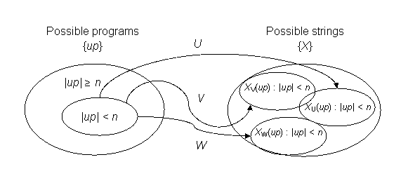 |
For the set of input strings where |up| < n, each UTM must map no more than 2n strings in {X} thanks to the Pigeonhole Principle. The target regions in {X} for U, V, and W may or may not overlap. They don't have to. Since we have an infinite number of UTMs to choose from, we can imagine that any mapping is possible, and this can in fact be demonstrated.
First, consider the following type of Turing Machine: it reads an input program p as a number, which its state table uses to begin a sequence. Each step in the sequence outputs a symbol without further reference to the program tape or the work tape, then halts. This implements a table look-up. If the TM reads N different numbers, it can output N different strings of arbitrary length. We could build a TM that outputs strings after reading 2-bit programs as follows:
|
Input Program |
Output String |
|
00 |
1011100001001111001 |
|
01 |
1010 |
|
10 |
0000011110110 |
|
11 |
1 |
The smallest size of table is, of course, a table with one entry, so with this type of Turing Machine we can output any string with a program 1 bit long.
There really is no limit to the length of the output string for a look-up table TM. We simply need a large enough table, which brings us to the following problem: the size of the look-up table exceeds its longest string. In other words, we would generally expect the string needed to describe the TM to be much longer than any string it can produce. That is where selection of UTM becomes critical.
The issue is, how do we code the selection of TM to run on the UTM? Since the description of our TM on the UTM is a string, it is also a number. The UTM will run TM 1, TM 2, TM 3, … TM N etc. depending on which number is loaded into the UTM. We can design a UTM to bounce just about anywhere in its state table when it reads the TM descriptor u, so any mapping from u to the TM implemented is possible. In fact, we could again use table look-up.
We will design a UTM called MFTM, or My Favorite Turing Machine. MFTM has a divided state and action table. The first part is dedicated to a single built-in implementation of a TM, whichever one we decide is our favorite. The other part implements any other arbitrarily chosen UTM Z. MFTM reads input string <a><q>. If a is a 0, it runs q on the built-in TM. If a is any other symbol, it runs <q> = <z><p> on Z, where z is a descriptor of a TM on Z and p is a program.
If we build in a table look-up TM in MFTM, it can produce arbitrary sequences from very short inputs. The shortest program on MFTM would be 2 bits if we embed a 1-entry table. MFTM doesn't violate the Pigeonhole Principle, because any <u><p> on Z must be lengthened by 1 bit on MFTM. The KC of every string not built into the table goes up by 1 bit.
Now this is admittedly a sneaky way to get low Kolmogorov Complexity for any arbitrary string, but it does illustrate the problem. Since we have an infinite number of UTMs, and there is an infinite number of ways to code TM descriptors on UTMs, including self-delimiting codes for which some descriptors are inherently short, there exist UTMs for which arbitrary sets of finite strings are not algorithmically random. This is important, because it demonstrates how strongly KC can depend on selection of UTM. The descriptor of the UTM is not included in calculating KC.
It is also possible to design a UTM on which strings have arbitrarily large KC. We will design a UTM called RIM, or Really Inefficient Machine. It will use a self-delimiting code to describe TMs, and this code is going to have the worst efficiency we can invent. Rather than coding 0 as 00, 1 as 11, and end as 01, we will code 0 as a successive string of n 0's, 1 as a successive string of n 1's, and end as any other substring of length n. We can make n very big, like 1020. Even though we might code T as u with q bits, RIM can't load T in less than nq bits. That means nq is a lower bound for KC on RIM.
This is a sneaky way to get high Kolmogorov Complexity for any arbitrary string, but again, it illustrates the problem. RIM doesn't violate the upper bound on KC or the Invariance Theorem, because we can let the constant c get very large. In fact, we have artificially done so.
Chaitin's Halting Probability: Ω(Omega)[Top]
Chaitin extended the work of Turing by defining the halting probability. Considering programs on a universal Turing machine U that require no input, we define P as the set of all programs on U that halt. Let |p| be the length of the bit string encoding program p, which is any element of P. The halting probability or Ωnumber is defined:
Ω= ∑2-|p| over all p elements of P
Again, the absolute value notation |p| denotes the size or length of the bit string p.
One way to think about Ωis that, if you feed a UTM with a random binary string generated by a Bernouli 1/2 process (such as tossing a fair coin) as its program, Ωis the probability that the UTM will halt.
As a probability, Ωhas a value between 0 and 1. Chaitin showed that Ωis not only irrational and transcendental, but is an uncomputable real number. It is algorithmically irreducible or algorithmically random no matter what UTM you pick. No algorithm exists that will compute its digits.
References[Top]
[1] Chaitin, G.J., Algorithmic Information Theory. Third Printing, Cambridge University Press, 1990. Available on-line.
[2] Turing, A.M., On Computable Numbers, with an Application to the Entscheidungsproblem. Proceedings of the LondonMathematical Society, ser. 2. vol. 42 (1936-7), pp.230-265; corrections, Ibid, vol 43 (1937) pp. 544-546. Available on-line.
[3] at the SEP, Editors, " Turing Machine", The Stanford Encyclopedia of Philosophy (Spring 2002 Edition), Edward N. Zalta(ed.), URL =< http://plato.stanford.edu/archives/spr2002/entries/turing-machine/>
[4] Hilbert, D., Mathematical Problems: Lecture Delivered before the International Congress of Mathematicians at Paris in 1900, translated by Maby Newson, Bulletin of the American Mathematical Society 8 (1902), pp. 437-479. , HTML version by D. Joyce available on-line.
[5] Gödel, K., On Formally Undecidable Propositions of Principia Mathematica and Related Systems. Monatshefte für Mathematik und Physik, 38 (1931), pp. 173-198. Translated in van Heijenoort: From Frege to Gödel. Harvard University Press, 1971.
[6] Copeland, B. Jack, " The Church-Turing Thesis", The Stanford Encyclopedia of Philosophy (Fall 2002 Edition), Edward N. Zalta(ed.), URL = < http://plato.stanford.edu/archives/fall2002/entries/church-turing/>.
[7] Hodges, Andrew, "Alan Turing", The Stanford Encyclopedia of Philosophy (Summer 2002 Edition), Edward N. Zalta(ed.), URL = <http://plato.stanford.edu/archives/sum2002/entries/turing/>.
[8] Minsky, M., "Size and Structure of Universal Turing Machines," Recursive Function Theory, Proc. Symposium. in Pure Mathematics, 5, American Mathematical Society, 1962, pp. 229-238.
[9] Rogozhin, Y. "Small Universal Turing Machines." Theoretical Computer Science 168 iss. 2, 215-240, 1996.
[10] Wolfram, S. A New Kind of Science. Champaign, IL: Wolfram Media, pp.706-711, 2002.
[Top]